Data Analysis with Python

Alright, Chef here! Let’s whip up this “Data Analysis with Python” dish.

Main Dish (Idea): Zesty Data Insights

The project aims to clean, explore, and extract insights from different datasets using Python and the Pandas library. It’s like creating a complex sauce where we want to understand the flavors and how they blend.

Ingredients (Concepts & Components):

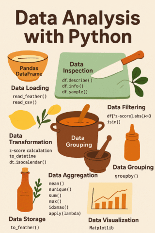
• Pandas DataFrame: The foundation – the mixing bowl where we hold our data.
• Data Loading (read_feather, read_csv): The process of gathering ingredients, fetching data from local feather files or online CSV repositories.
• Data Inspection (df.describe(), df.info(), df.sample()): Tasting and smelling the raw ingredients to understand their basic properties (like mean, standard deviation, missing values, and a sneak peek at the data).
• Data Transformation (z-score calculation, to_datetime, dt.isocalendar()): Chopping, seasoning, and preparing the ingredients.
• Data Filtering (df[‘z-score’].abs()<=3, isin()): Sorting out the bad apples by removing outliers.
• Data Grouping (groupby()): Combining ingredients based on shared characteristics, like simmering different herbs together.
• Data Aggregation (mean(), nunique(), sum(), max(), idxmax(), apply(lambda)): Extracting key flavors from each group, like reducing a sauce to concentrate its taste.
• Data Storage (to_feather()): Saving prepared ingredients (DataFrames) for later use.
• Data Visualization (Matplotlib): The artistic plating, plotting some data for better visual exploration
• Z-score: One of the spices, outlier detection
• Ad Campaign Analysis: Crunching some ads for a hypothetical ad agency and reporting their ID + total spend

Cooking Process (How It Works):

1. Gather the Ingredients: Load data from CSV files (using pd.read_csv) or pre-existing feather files (using pd.read_feather) into Pandas DataFrames.
2. Taste the Ingredients: Perform basic EDA using .describe(), .info(), and .sample() to understand the data’s shape and contents.
3. Prepare the Ingredients: Clean and transform the data:
   • Calculate Z-scores to identify outliers.
   • Convert date columns to DateTime objects.
   • Extract week numbers from dates.
4. Combine and Simmer: Use the groupby() function to group data based on columns like country, year, or continent. Then, use aggregation functions like .mean(), .nunique(), .sum(), and custom lambda functions.
5. Adjust the Flavor: Identify and remove outliers.
6. Reduce and Concentrate: Use the aggregation and transformation steps to find specific insights. For example, find the advertiser with the highest spend or the relationship between continent, year, population, and per capita GDP.
7. Preserve for Later: Save results, particularly transformed DataFrames, to feather files for faster loading in future sessions.
8. Plating: The Gapminder data is plotted (if there is the year of > 2010) to visualize how GDP changed overtime per country.

Serving Suggestion (Outcome):

A cleaned, explored, and insightful dataset is served, ready for further analysis and modeling. For example:

• A Gapminder dataset, ready for time-series forecasting or geographical plotting.
• Identification of which advertisers are using the most unique and high value ad strategies.
• A deeper understanding of global trends in life expectancy, population, and GDP.

Bon appétit!